ST790 Advanced Computing Lab: Introduction to CVX

This file demonstrates how to use the modeling tool CVX to solve optimization problems, and also includes some examples of using MATLAB's and Gurobi's solvers directly. It was originally created by Brian Gaines for Eric Chi's ST790 Advanced Computing at NC State University. The companion slidedeck provides additional information on CVX. The code that generated this file is available (cvxDemo.m). Any comments or suggestions are welcome.

This file requires:

MATLAB's Optimization Toolbox (if you are an NCSU student, you have this)
The CVX toolbox for disciplined convex optimization (preferrably with the professional license)
cvxDemo.mat data file in the working directory (or the load path will need to be changed)
A stand-alone installation of the Gurobi solver is optional. If you do not have a stand-alone installation of Gurobi, please change the gurobiInstalled string to equal 'no' so the Gurobi-related code will be skipped.

Initial Setup
Linear Programming Example: $\ell_1$ regression (least absolute deviations)
LP Example: Linprog
LP Example: Gurobi
LP Example: CVX
Quadratic Programming Example: Lasso Regression
QP Example: Quadprog
QP Example: Gurobi
QP Example: CVX
Additional Example: 1-norm SVM

Initial Setup

% clean up workspace
clear;

%######## Does this machine have a stand-alone Gurobi installation?? ########%
% Answer 'yes' or 'no'
gurobiInstalled = 'yes';

% load data
load('cvxDemo')

Linear Programming Example: $\ell_1$ regression (least absolute deviations)

The first example is $\ell_1$ regression. As the name suggests, this is similar to the typical regression setup except that the $\ell_1$ norm is used for the loss function, so the objective function becomes

minimize $|| y - X\beta ||_1$

To solve this using a linear programming solver, we need to put it in the solver's standard form (which may differ slightly from the standard form Dr. Chi presented in class).

LP Example: Linprog

For MATLAB's lingprog function, we see that (from the online documentation or by the command "help linprog" in MATLAB) the problem's form is given by

minimize $f'x$

subject to $Ax \le b$ , $Aeq \cdot x = beq$ , and $lb \le x \le ub$ .

Once we massage the problem into this form (I will do this on the board), then the corresponding function call is:

x = linprog(f, A, b, Aeq, beq, lb, ub, x0, options);

Not all of the inputs are required. For example, if we only have linear inequaltiy constraints, the function call becomes

x = linprog(f, A, b);

If some of the intermediate function inputs are not needed, they need to be replaced by two square brackets, []. So if we had linear equality constraints but no linear inequality constraints, the code is

x = linprog(f, [], [], Aeq, beq);

Anyway, after massaging the $\ell_1$ regression problem into this form, we can translate it to the code:

$x = \theta = \pmatrix{\beta \cr r}$

$f = \pmatrix{0_p \cr 1_n}$

f = [zeros(p1, 1); ones(n1, 1)];

$A = \pmatrix{X & -I_n \cr -X & -I_n}$

A = [X1 -speye(n1); -X1 -speye(n1)];

$b = \pmatrix{y \cr -y}$

b = [y1; -y1];

$\beta \in \mathcal{R}^p$ , and $r \ge 0_n$

lb = [-inf(p1, 1); zeros(n1, 1)];

Now that all of the inputs are set, we can call lingprog to estimate the parameters, then extract the first $p$ parameters as those correspond to $\hat{\beta}$ .

tic;                                            % start timer
thetaHatLP = linprog(f, A, b, [], [], lb);      % estimate parameters
toc;                                            % run time
betaHatLP = thetaHatLP(1:p1);                   % extract estimates for beta

Optimization terminated.
Elapsed time is 0.522778 seconds.

LP Example: Gurobi

Please note that this requires a standalone installation of Gurobi, which is free for academic users but was not required for this lab. However, I do encourage the knowleddge of a commercial solver such as Gurobi or MOSEK (both of which are free for academic users, follow the links) as those are state-of-the-art solvers and more efficient than MATLAB's built-in solvers and the R equivalents that I'm aware of (both Gurobi and MOSEK are available in R).

As before, the first thing we need to do is become familiar with what the standard form looks like according to the solver. A quick view of this is available through Gurobi's online documentation, while the details are available in the actual reference manual (p. 433). The relevant parts for our purposes are

minimize $x'Qx + c'x + alpha$

subject to $Ax = b$ and $l \le x \le u$ .

and the function call is

gurobi(model, params)

For Gurobi, the model argument is pieced together in a struct variable (which is essentially like a list in R) that contains different fields that correspond to the various parts of the optimization poblem. The field of a struct is referenced with a period, so the syntax is struct.field.

Here are a few notes on constructing the model, as the implementation is not as straightforward as linprog:

is required (so a vector of zeros is used if it is not needed), and obj is its corresponding field (model.obj)
is also required, and it must be a sparse matrix (using the sparse function). Even if you do not have any constraints in your model, is still required and has to be sparse (so simply using [] doesn't work). As we will see in the lasso example, I usually use sparse(zeros(0, p));, where is the dimension of the parameter vector/optimization variable, to create a sparse empty matrix.
Linear inequality constraints are also possible, even though the standard form only has linear equality constraints. The sense field specifies the type of constraint, using either '=', '<', or '>'. A single value can be used when all of the constraints are the same, otherwise for mixed constraints there needs to be one value per row of . Since A is required, sense is also required.
The field for is rhs. This is also required.
The field for is lb. This is optional, but please note that the default lower bound is zero, and not $-\infty$ , which can be accomplished by using -inf(p, 1).
params is optional and can be used to specify options. A list of options is available on page 487 of the reference manual. I typically only set the field OutputFlag to to suppress the output.
x is the field in the output struct that has the solution. The solution includes several other output fields, detailed on p. 436 of the referencec manual.

Now that we have some background on gurobi, we can see it in action:

%# Model Setup #%
% linear term
gmodel.obj = [zeros(p1, 1); ones(n1, 1)];
% constraint matrix
gmodel.A = [X1 -speye(n1); -X1 -speye(n1)];
% constraint type. Only one value needed since all constraints are inequality
gmodel.sense = '<';
% b vector for constraints
gmodel.rhs = [y1; -y1];
% lower bound (needed because default is zero)
gmodel.lb = [-inf(p1, 1); zeros(n1, 1)];
% suppress output
gparam.OutputFlag = 0;

%# Model Estimation #%
if strcmpi(gurobiInstalled, 'yes')
    tic;                                    % start timer
    gresult = gurobi(gmodel, gparam);       % estimate model
    toc;                                    % run time
    betaHatGurobiLP = gresult.x(1:p1);      % extract estimates for beta
end

Elapsed time is 0.007671 seconds.

LP Example: CVX

While Gurobi and MOSEK are solvers, CVX is a modeling tool which provides a much more user-friendly interface for solving optimization problems using a variety of solvers, saving the hassle of needing to massage the problem into standard form or the hassle of having to learn each solver's syntax.

I will get into the details of CVX later, but for now, let's look at how we would solve the $\ell_1$ regression problem using CVX.

%# Model Estimation #%
tic;                                             % start timer
cvx_begin quiet                                  % initiate CVX, hiding output
    variable betaHatCVX_LP(p1);                  % declare optimization variable
    minimize( norm(y1 - X1*betaHatCVX_LP, 1) );  % define objective function
cvx_end                                          % declare end of CVX statements
toc;                                             % run time

As you can see, the syntax is much more straightforward and succinct, and essentially translates the original form of the problem directly to code without first having to massage it into an intermediate form for the sake of estimation. Here

%# Compare estimates #%
% reduce the number of decimals displayed
format short
% display estimates
if strcmpi(gurobiInstalled, 'yes')
    display([betaHatLP betaHatCVX_LP betaHatGurobiLP])
elseif strcmpi(gurobiInstalled, 'no')
    display([betaHatLP betaHatCVX_LP])
end

Elapsed time is 0.564291 seconds.

ans =

   -0.5722   -0.5722   -0.5722
    0.5249    0.5249    0.5249
    0.6711    0.6711    0.6711
   -0.0283   -0.0283   -0.0283
    0.1598    0.1598    0.1598
    0.8119    0.8119    0.8119
   -0.1091   -0.1091   -0.1091
    0.2011    0.2011    0.2011
    0.0029    0.0029    0.0029

Quadratic Programming Example: Lasso Regression

Our second example involves the popular Lasso (Tibshirani, 1996), which introduces an $\ell_1$ penalty term on the regression coefficients in the objective function

minimize $|| y - X\beta ||_2^2 + \lambda || \beta ||_1$

where $\lambda \ge 0$ is a tuning parameter.

We will first optimize this directly using both MATLAB's solver (quadprog) and Gurobi, which will require us to first transform the problem into each solver's standard form.

QP Example: Quadprog

MATLAB's quadprog function naturally extends the lingprog function to include a quadratic term (documentation):

minimize $\frac{1}{2}x'Hx + f'x$

subject to $Ax \le b$ , $Aeq \cdot x = beq$ , and $lb \le x \le ub$ .

and the function call is also similar

x = quadprog(H, f, A, b, Aeq, beq, lb, ub, x0, options);

The key trick to reformulating our problem is to represent the parameter vector using its positive and negative parts, $\beta = \beta^+ - \beta^-$ , as this allows us to deal with the absolute value in the penalty term, since $|\beta| = \beta^+ + \beta^-$ . After expanding and rearranging the objective function to match quadprog's standard form, it should look like

$\frac{1}{2} \pmatrix{\beta^+ \cr \beta^-} ' \pmatrix{X'X & -X'X \cr -X'X & X'X} \pmatrix{\beta^+ \cr \beta^-} + \left( \lambda 1_{2p} - \pmatrix{X'y \cr -X'y} \right)' \pmatrix{\beta^+ \cr \beta^-}$

subject to $\beta^+ \ge 0$ , $\beta^- \ge 0$

so we can now translate this to code:

%# Model Setup #%
% Quadratic matrix H
gram = X2'*X2;
H = [gram -gram; -gram gram];
% constraints
lb2 = zeros(2*p2, 1);
% constant part of linear coefficient f
Xy2 = X2'*y2;
f2p2 = [Xy2; -Xy2];
% suppress quadprog output
options = optimset('Display', 'off');

%# Model Estimation #%
% define grid of tuning parameters
lambdas = (0:2:64);
nLambda = length(lambdas);

% matrix to store parameter estimates
betaHatPathQP = NaN(p2, nLambda);
% vector to store estimation time
qpTimerPath = NaN(1, nLambda);

% estimate model using quadprog, looping over lambdas
for k = 1:nLambda
    % finish constructing f
    f2(1:2*p2, 1) = lambdas(k);
    f2 = f2 - f2p2;

    % estimate model using quadprog
    tic;
    thetaHatQP = quadprog(H, f2, [], [], [], [], lb2, [], [], options);
    qpTimer = toc;

    % back out estimates of beta
    betaHatPathQP(:, k) = thetaHatQP(1:p2) - thetaHatQP(p2+1:end);
    % store estimation time
    qpTimerPath(k) = qpTimer;
end

QP Example: Gurobi

Gurobi's standard formulation already inludes a quadratic term,

minimize $x'Qx + c'x + alpha$

subject to $Ax = b$ and $l \le x \le u$ ,

so we can proceed as before while also including the quadratic matrix, $Q$ , which is required to be sparse.

%# Model Setup #%
% quadratic matrix
gram = X2'*X2;
gmodel2.Q = sparse([gram -gram; -gram gram])/2;
% constant part of linear term f
Xy2 = X2'*y2;

Recall from above that $A$ and $b$ are required, even if they are not in our model, and that $A$ has to be a sparse matix (p. 433-4 of the reference manual). So we will create $A$ as a sparse, empty matrix and $b$ as an empty vector. Note that $A$ 's dimensions still need to be conformable, but $b$ can be a 0-by-1 vector.

% Constraint matrix.  This is an empty matrix since it's not in our problem
gmodel2.A = sparse(zeros(0, 2*p2));
% constraint type
gmodel2.sense = '=';
% right hand side of constraints (corresponds to b), also empty
gmodel2.rhs = zeros(0, 1);
% suppress gurobi output;
gparam.OutputFlag = 0;


%# Model Estimation #%
if strcmpi(gurobiInstalled, 'yes')
    % matrix to store parameter estimates
    betaHatPathGurobi = NaN(p2, nLambda);
    % vector to store estimation time
    gurobiTimerPath = NaN(1, nLambda);

    % solve model, looping over lambdas
    for k = 1:nLambda
        % update linear coefficient
        gmodel2.obj = lambdas(k)*ones(2*p2, 1) - [Xy2; -Xy2];

        % estimate model using Gurobi
        tic;
        gresult = gurobi(gmodel2, gparam);
        gurobiTimer = toc;

        % store estimated coefficients
        betaHatPathGurobi(:, k) = gresult.x(1:p2) - gresult.x(p2+1:end);
        % store estimation time
        gurobiTimerPath(k) = gurobiTimer;
    end
end

QP Example: CVX

To solve the lasso in CVX, the implementation is again more straightforward as we can work directly the original formulation. The core part of the estimatin code is given by

   cvx_begin quiet
       variable betaHatCVX_QP(p);
       minimize( 0.5*sum_square(y - X*betaHatCVX_QP) + ...
           lambda*norm(betaHatCVX_QP, 1) );
   cvx_end

So to solve the problem n a grid of $\lambda$ values, we can loop over this as

%# Model Estiation #%
% matrix to store parameter estimates
betaHatPathCVX = NaN(p2, nLambda);
% vector to store estimation time
cvxTimerPath = NaN(1, nLambda);

% solve model, looping over lambdas
for k = 1:nLambda
    % estimate model using CVX
    tic;
    cvx_begin quiet
        variable betaHatCVX_QP(p2);
        minimize( 0.5*sum_square(y2 - X2*betaHatCVX_QP) + ...
            lambdas(k)*norm(betaHatCVX_QP, 1) );
    cvx_end
    cvxTimer = toc;

    % store estimated coefficients
    betaHatPathCVX(:, k) = betaHatCVX_QP;
    % store estimation time
    cvxTimerPath(k) = cvxTimer;
end

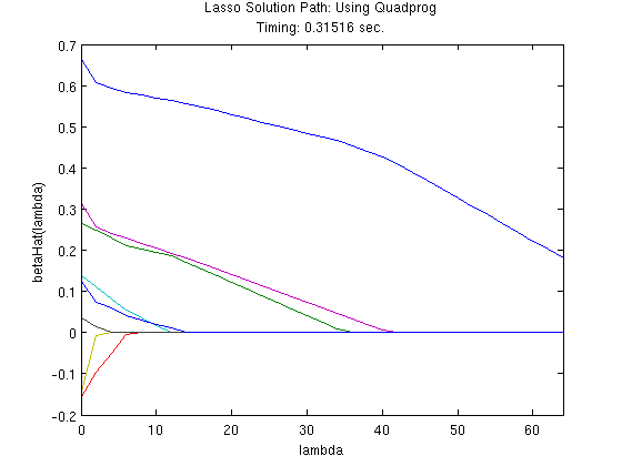
%# Plot solutions #%
% Quadprog
figure;
plot(lambdas, betaHatPathQP);
title({'Lasso Solution Path: Using Quadprog', ...
    ['Timing: ' num2str(sum(qpTimerPath)) ' sec.'] })
xlabel('lambda');
ylabel('betaHat(lambda)');
xlim([min(lambdas), max(lambdas)]);

% Gurobi
if strcmpi(gurobiInstalled, 'yes')
    figure;
    plot(lambdas, betaHatPathGurobi);
    title({'Lasso Solution Path: Using Gurobi', ...
        ['Timing: ' num2str(sum(gurobiTimerPath)) ' sec.'] })
    xlabel('lambda');
    ylabel('betaHat(lambda)');
    xlim([min(lambdas), max(lambdas)]);
end

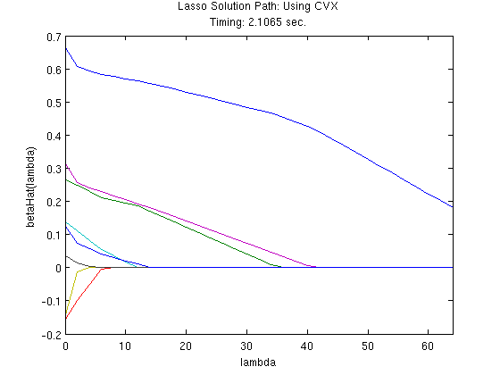
% CVX
figure;
plot(lambdas, betaHatPathCVX);
title({'Lasso Solution Path: Using CVX', ...
    ['Timing: ' num2str(sum(cvxTimerPath)) ' sec.'] })
xlabel('lambda');
ylabel('betaHat(lambda)');
xlim([min(lambdas), max(lambdas)]);

Additional Example: 1-norm SVM

Here is an additional example of using CVX, this time for solving a 1-norm SVM (Zhu et al., 2004), which is given by

minimize $\sum_{i = 1}^n \left[1 - y_i \left(\beta_0 + \sum_{j=1}^p x_{ij} \beta_j \right) \right]_+$

subject to $|| \beta ||_1 =\sum_{j=1}^p \beta_j \le t$ ,

where $s \ge 0$ is a tuning parameter. This example involves a function, the hinge loss function, that is not already in the CVX function library. However, we can quickly define a new function for this purpose, and since it follows the DCP ruleset, CVX can identify it as being convex.

% define function handle for hinge loss
hingeLoss = @(x) sum(max(0, 1 - x));

With this in hand, the core part of the estimation code is

   cvx_begin quiet
       variable betaHatSVM(p3);
       minimize( hingeLoss(y3.*(X3*betaHatSVM)) );
       subject to;
           norm(betaHatSVM(2:end), 1) <= tValues(k);
   cvx_end

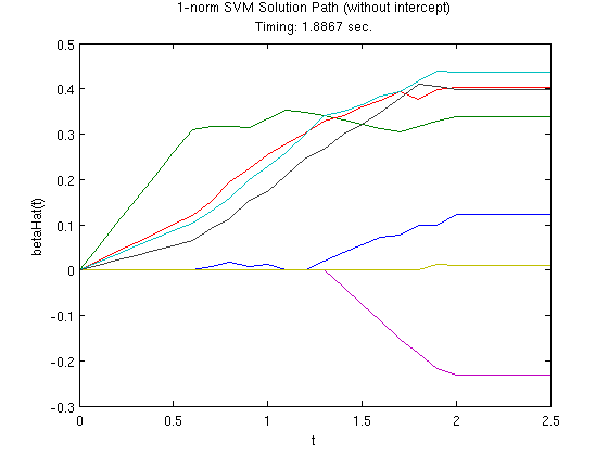
%# Model Estiation #%
% create tuning parameter grid
tValues = (0:0.1:2.5);
% number of tuning parameters to consider
m = length(tValues);

% matrix to store parameter estimates
betaHatPath3 = NaN(p3, m);
% vector to store estimation time
svmTimerPath = NaN(1, m);

% solve model, looping over lambdas
for k = 1:m
    % estimate model using CVX
    tic;
    cvx_begin quiet
        variable betaHatSVM(p3);
        minimize( hingeLoss(y3.*(X3*betaHatSVM)) );
        subject to;
            norm(betaHatSVM(2:end), 1) <= tValues(k);
    cvx_end
    % store estimation time
    svmTimerPath(k) = toc;

    % store estimated coefficients
    betaHatPath3(:, k) = betaHatSVM;
end


% #Plot solution path #%
figure;
plot(tValues, betaHatPath3(2:end, :));
title({'1-norm SVM Solution Path (without intercept)', ...
    ['Timing: ' num2str(sum(svmTimerPath)) ' sec.'] })
xlabel('t');
ylabel('betaHat(t)');
xlim([min(tValues), max(tValues)]);